This post is meant as a total beginner’s intro to LAMMPS, the molecular dynamics simulation software, and assumes very little prior knowledge of MD simulation. It’s been a few years since I’ve worked on this, but I remember how overwhelming it felt trying to learn about LAMMPS and piece together all of the relevant information to actually be able to run a simulation, so hopefully I can help to ease that process for someone else.
Resources
I’ve found the official LAMMPS docs to be quite good. It’s a bit overwhelming at first and you might have to read through it multiple times, but I think you’ll find it to be well written.
Also, the examples (docs, code) are very helpful to gain a practical example of how to run a simulation.
Overview
If you look at the peptide example, you’ll find two important files: the input script (in.peptide) and the data file (data.peptide).
Brief aside: For some strange reason, LAMMPS files tend to be named with the file extension first as opposed to the normal convention of putting the extension at the end.
It’s as if you had named a photo jpg.myface instead of myface.jpg.
This is totally optional, the file extension is only a hint to tell the user what the file contains.
You can name your input and data files however you want, and as long as you use the same name in your code, it will work fine.
The input script contains your instructions for LAMMPS describing all the details of your simulation.
On Line 13, you’ll see read_data data.peptide, which loads the data file, which contains the initial positions, bonds, etc. of your atoms.
So the input script describes how to run the simulation, and the data file describes what you’re simulating.
Input script (docs)
Other commands in the peptide example input script:
- L3-4 describes the physical units for all values and some details about the atom model.
- L6-10 describes what functions are used to calculate the interaction between atoms (see e.g. pair_style lj/charmm/coul/charmm, which describes a specific version of the important Lennard-Jones potential)
- L15-16 describes the neighbor list, which allows the simulation to run much faster by ignoring interactions between atoms that are too far apart, and only updating the list periodically.
- L18 specifies the time precision of the simulation. Smaller time steps make the simulation more accurate, but takes longer to finish.
- L41 specifies the number of time steps to run, basically the time duration of your simulation
- L20-24 are perhaps the most complicated but important. These determine the thermodynamics of your simulation, which describe the macroscopic conditions your simulation exists within. I was lucky that my professor set this for me and I didn’t have to worry about it. But if you have to set these parameters yourself, you’ll have to study statistical mechanics to determine what kind of ensemble you need.
- L28-36 determine what kind of files LAMMPS should produce as it runs. The important one is L28, which specifies that the positions and velocities of all atoms should be written to a text file (
dump.peptide) every 10 timesteps. The dump file (a.k.a.lammpstrj) is the final output of the simulation that you will later analyze.
You might also find write_restart, which is like a checkpoint in case you need to stop and resume your simulation. This is important since they can take days or weeks to complete. A restart file generally contains more information than the dump file, and is stored as a binary file rather than a text file, so it’s not suitable for analyzing your simulation as you would analyze the dump file to gain insight from your simulation.
Data file (docs)
The data file describes the atoms, their interactions, and their initial positions. The most common interactions are bonds (2 atoms apply forces on each other as a function of distance) and angles (forces applied on three atoms connected by two bonds as a function of the angle between the bonds). You can see both depicted here:

There are also other interactions, including dihedrals and impropers, which act on groups of more than 3 atoms.
Note that these interactions (angles, bonds, dihedrals, impropers) are permanent and unbreakable. If a bond exists between two specific atoms, it will continue to exist for the whole simulation. Also keep in mind that a bond does not constrain two atoms to always be an exact distance apart. Rather, it strongly encourages them to maintain that distance by applying forces on them.
However, there are also transient interactions between atoms, primarily the pairwise electrostatic interaction described the Lennard-Jones potential specified in the pair_style command in the input script. This force is only applied between two atoms if they are close enough to be considered neighbors on the neighbor list. If they move away from each other during the simulation, they will no longer interact electrostatically.
Header
- The first section of the file (L1-13 in
data.peptide) describes the contents of the file. These should match the number of entries in each section below. - L15-17 describes the bounding box of the simulation. The universe is huge, and the bounding box describes the tiny part of it that you’re simulating. The boundary conditions can be set in the input file via the
boundarycommand. You might use a periodic box to simulate a large quantity of something, or a fixed boundary (hard wall) in other situations.
Atom sections
Every atom has a type, which generally corresponds to an element. So all of your oxygen atoms might be type 1, and your hydrogen atoms might be type 2. However, if you have oxygen atoms in both your droplet and your substrate, you might choose to give them different types to capture the fundamentally different way they interact with other atoms.
In the Masses section (L19-34), there are two columns: the first one is the type, and the second one is the mass. So e.g. every atom of type 1 has a mass of 12.0110 (in whatever units are specified by the units command in the input script).
In the Atoms section (L137-2142), each individual atom is described. Each atom has a unique id which differentiates it from all other atoms. The columns depend on the atom_style specified in input script. Refer to the table in the Atoms section of the data file reference for details. In this example, we have atom_style full, so the columns are:
- atom-ID
- molecule-ID
- atom-type
- q (charge)
- x (initial)
- y (initial)
- z (initial)
Similarly, the Velocities section (L2144-4149) lists the initial x, y, and z components of velocity for each atom (again, the first column is atom-id).
Coefficient sections
Just like we have “types” of atoms, we have “types” of bonds which are different from one another. Just like the Masses section lists the mass for each type of atom, the other Coeff sections give parameters for each type of interaction. Similar to the Atoms section, the meaning of the parameters in each section depends on the interaction style defined in the input file. We can look up the order and meaning of the parameters on the docs page for that specific interaction style.
All of these interaction parameters are generally determined experimentally, so if you’re just working on a simulation, you’ll have to find published values for your specific materials. In my case, I found the parameters necessary to create a mica substrate from the INTERFACE force field.
For example, take the Bond Coeffs section (L53-72). In the input script, we have bond_style harmonic. The bond_harmonic doc page gives the equation for the force applied on each atom due to a harmonic as a function of the distance between the atoms as
E = K(r - r_0)^2and lists the parameters in order as:
K(energy/distance^2)r_0(distance)
So, the first entry in the Bond Coeffs section is
1 249.999999 1.490000which creates a bond with
type = 1K = 249.999999r_0 = 1.490000
The Angle Coeffs, Dihedral Coeffs, and Improper Coeffs similarly create interaction types with the specified parameters.
Pair Coeffs section
However, the Pair Coeffs section is special in that the pairs coefficients are defined for each atom type.
So if you have 14 atom types, then you must also have 14 lines in the Pair Coeffs section.
This is because unlike other interactions which only occur between specific atoms,
electrostatic interactions can occur between any two atoms that are sufficiently close to one another,
and the interaction depends only on the type of the atoms involved.
In the peptide example, we have
pair_style lj/charmm/coul/long 8.0 10.0 10.0and the pair_charmm doc page says that we therefore need to define the following pair coeffs for each atom:
ϵ(energy units)σ(distance units)ϵ_14(energy units) (optional)σ_14(distance units) (optional)
and the first entries in the Pair Coeffs section is
  1    0.110000    3.563595    0.110000    3.563595
  2    0.080000    3.670503    0.010000    3.385415
So if two atoms of type 1 are sufficiently close, they will each feel a lennard jones force as a function of their distance, with ϵ = 0.110000, σ = 3.563595, etc.
And two atoms of type 2 would interact with ϵ = 0.110000 and σ = 3.563595.
But what happens when an atom of type 1 has a pairwise interaction with an atom of type 2? The answer is that their interaction is defined by coefficients determined through mixing rules, as specified in detail in the relevant LAMMPS docs. Basically, a special average of the individual pure coefficients is used to determine the coefficients of the mixed interaction.
Interaction sections
The final important section of the data file is the interaction sections, called Bonds, Angles, etc., where the specific bonds, angles, etc. among our atoms are actually defined. This is the simplest part of the file.
- The first column is a unique interaction id
- The second column is the interaction type
- The remaining columns are the unique ids of the atoms involved in the relationship.
For example the first line of the Bonds section (L4151-5517) is
1 3 1 7This creates bond #1 with type #3 between atom #1 and atom #7.
Since bonds are symmetric, the order of the atoms doesn’t matter. It would be equivalent to write
1 3 7 2However, the order is significant in the other non-pairwise interactions.
For example, the Angles section of the read_data docs says
The 3 atoms are ordered linearly within the angle. Thus the central atom (around which the angle is computed) is the atom2 in the list. E.g. H,O,H for a water molecule.
Visualization
You can see that in the peptide input script, they are also dumping .jpg and .mpg files. I don’t recommend this. LAMMPS is great for simulation, but it produces very ugly images/movies. For visualization, use VMD, which you can use interactively or automatically to create beautiful images like this:
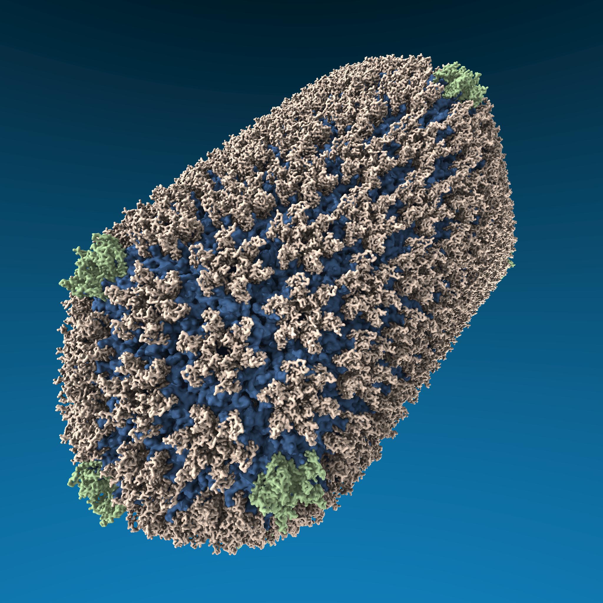
VMD can load your LAMMPS dump file directly using the readlammpsdata command.
Post-analysis
Assuming that you’re not just running simulations to make pretty pictures, you’ll want to perform some kind of post-analysis on the results of your simulation. This is highly problem-dependent, and you’re likely going to have to write a bunch of code from scratch to calculate the exact thing you’re interested in. You’ll do this by parsing the dump file, which is basically a huge text file (or set of files) with one line per atom per time step, and then running your custom calculations. Of course, you should search around first to see if someone else has already written code that would work for you, especially if you’re doing a routine calculation on a novel subject.
In my case, I was working on droplet wetting, and I wrote a C++ library using ROOT to detect the boundary of the droplet and analyze the change in geometry over time. If my code works for you, feel free to use it. Although like most free software, it comes with no warranty, and you may have to spend a fair amount of time trying to get it running on your machine with your data.
Good luck!
Hopefully this is enough to get you started running some exciting simulations. Feel free to email me if you’d like to discuss my work or yours.
Happy simulating!
— Oliver